2024. 8. 14. 15:48ㆍ머신러닝&딥러닝/생성모델
AutoEncoder는 전통적인 Encoder-Decoder 구조이다. 이 중 Variational AutoEncoder(VAE)는 Encoder q로 latent 분포의 평균과 분산을 샘플링하고, 이를 결합하여 latent space를 만드는 reparametrization trick을 이용한다.
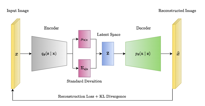
이러한 VAE는 latent vector가 주어지면 학습된 decoder로 새로운 이미지를 generation할 수 있다. 그렇다면, 잘 학습된 VAE의 latent space는 어떻게 생겼을까? 클래스가 구분된 input image를 latent로 보내면, latent 안에서도 클래스끼리 clustering이 되어 있을까?
본 포스팅에서는 https://github.com/Jackson-Kang/Pytorch-VAE-tutorial 에 나온 코드를 변형하여, MNIST 이미지들의 latent vector를 시각화하는 실험을 해 보았다.
GitHub - Jackson-Kang/Pytorch-VAE-tutorial: A simple tutorial of Variational AutoEncoders with Pytorch
A simple tutorial of Variational AutoEncoders with Pytorch - Jackson-Kang/Pytorch-VAE-tutorial
github.com
VAE.py
먼저, 모델 클래스에 self.latent라는 변수를 추가하여 latent를 저장할 수 있도록 하였고 이것의 getter 메소드를 만들었다. self.latent는 reparametrization 때 인스턴스에 저장된다.
class Model(nn.Module):
    def __init__(self, Encoder, Decoder):
        super(Model, self).__init__()
        self.Encoder = Encoder
        self.Decoder = Decoder
        self.latent = None

    def reparameterization(self, mean, var):
        epsilon = torch.randn_like(var).to(DEVICE)        # sampling epsilon
        z = mean + var*epsilon                          # reparameterization trick
        self.latent = z
        return z

    def getLatent(self):
        return self.latent

    def forward(self, x):
        mean, log_var = self.Encoder(x)
        z = self.reparameterization(mean, torch.exp(0.5 * log_var)) # takes exponential function (log var -> var)
        x_hat            = self.Decoder(z)

        return x_hat, mean, log_var
Training Loop
이 부분은 위 깃헙에서 변형하지 않고 진행하였다. CPU 환경에서 30 epoch 학습하는 데 약 3분 30초 걸렸다. Latent의 길이는 200이다. 즉 28by28 MNIST 이미지 한 장당 길이 200의 latent로 압축되는 것이다.

Inference
latents = []
with torch.no_grad():
    for batch_idx, (x, y) in enumerate(test_loader):
        x = x.view(batch_size, x_dim)
        x = x.to(DEVICE)
        x_hat, mean, log_var = model(x)
        latents.append((model.getLatent(), y))
latent가 저장되는 리스트를 만들고, (latent, 정답) 형태의 튜플로 test set에 있는 데이터를 저장해 주었다. 테스트 데이터는 10,000개가 batch size 100으로 나뉘어 들어간다.
Latent의 PCA
200 dim 짜리 latent vector를 3차원으로 PCA 해 주었다. 왜 3차원이냐, 2차원으로 해봤는데 뭉개진다. 그나마 클러스터가 잘 보이는 3차원으로 축소해 봤다.
import matplotlib.cm as cm


vectors = []
answers = []
for i in range(latents[0][0].shape[0]):
    vectors.extend([item[0].numpy()[i] for item in latents])
    answers.extend([item[1].numpy()[i] for item in latents])

vectors = np.array(vectors)
answers = np.array(answers)

pca = PCA(n_components=3)
projected_vectors = pca.fit_transform(vectors)


colors = cm.rainbow(np.linspace(0, 1, 10))


views = [(20, 60), (90, 0), (0, 90), (30, 45)]
view_titles = ['Default View', 'Top-down View', 'Side View', 'Diagonal View']

for i, (elev, azim) in enumerate(views):
    fig = plt.figure(figsize=(8, 6))
    ax = fig.add_subplot(111, projection='3d')

    for j in range(10):
        indices = np.where(answers == j)[0]
        ax.scatter(projected_vectors[indices, 0], projected_vectors[indices, 1], projected_vectors[indices, 2],
                   color=colors[j], label=f'Answer {j}', alpha=0.6)

    ax.view_init(elev=elev, azim=azim)
    ax.set_xlabel('PCA Component 1')
    ax.set_ylabel('PCA Component 2')
    ax.set_zlabel('PCA Component 3')
    ax.set_title(view_titles[i])
    ax.legend(loc='upper right')

    plt.show()
3차원 플롯을 네 방향에서 본 것으로 출력해 봤다.


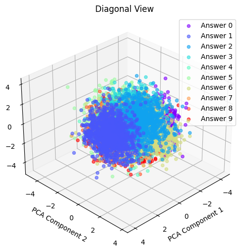
같은 숫자끼리는 어느 정도 유사한 위치로 클러스터가 생기는 것을 확인할 수 있다.
Random Sampling & Generation
이제, latent vector를 random sampling하고, 학습된 decoder로 복원하여 어떤 숫자가 나오는지 확인하자.
random_sample = np.random.randn(1, vectors.shape[1])
projected_random_sample = pca.transform(random_sample)[0]
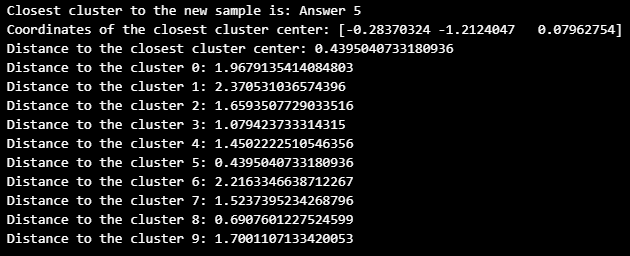
0~9 클러스터의 중심 좌표를 계산하고, Scipy를 이용하여 새로운 랜덤 latent와 가장 가까운 클러스터를 찾아 보았다.
from scipy.spatial.distance import cdist
cluster_centers = []
for j in range(10):
    indices = np.where(answers == j)[0]
    cluster_center = np.mean(projected_vectors[indices], axis=0)
    cluster_centers.append(cluster_center)

cluster_centers = np.array(cluster_centers)


distances = cdist(np.array([projected_random_sample]), cluster_centers, metric='euclidean')
closest_cluster_index = np.argmin(distances)
closest_cluster = closest_cluster_index

print(f"Closest cluster to the new sample is: Answer {closest_cluster}")
print(f"Coordinates of the closest cluster center: {cluster_centers[closest_cluster]}")
print(f"Distance to the closest cluster center: {distances[0, closest_cluster]}")

for i in range(10):
    print(f"Distance to the cluster {i}: {distances[0, i]}")
가장 가까운 클러스터는 5라고 한다.
이제 학습된 디코더로 latent를 이미지로 바꾸자.
lat = torch.tensor(random_sample).float().to(DEVICE)
generated_image = decoder(lat)


def show_image(x, idx):
    x = x.view(1, 28, 28)
    fig = plt.figure()
    plt.imshow(x[idx].detach().cpu().numpy())


show_image(generated_image, idx=0)
어? 5 아닌 것 같은데? 다른 것도 시도해 보았다.

몇 가지 샘플을 더 시도해 보았는데, 아래와 같이 가장 가까운 클러스터의 샘플과 generation된 결과는 같지 않았다.
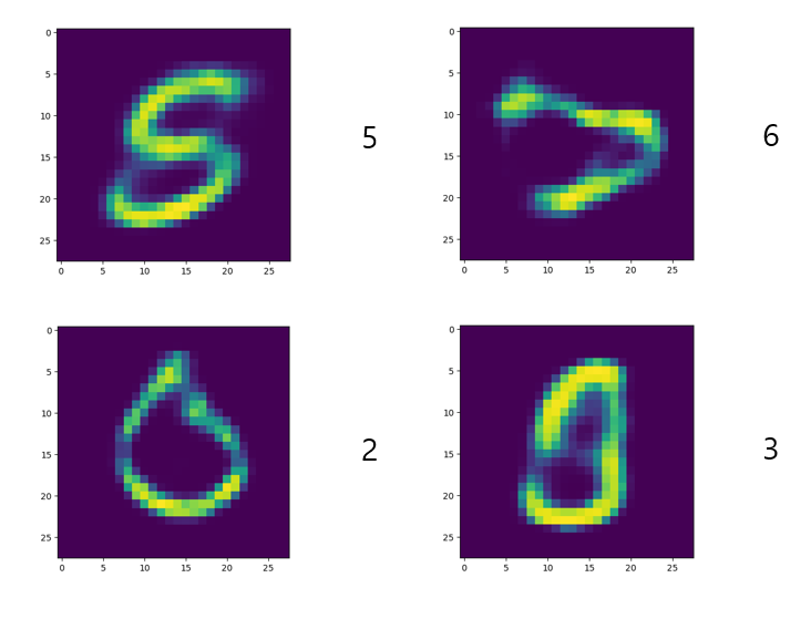
다른 분들과 논의해본 결과, Latent vector가 PCA를 통해 clustering될 수는 있지만, 그렇게 구분된 클러스터가 class에 대한 decision boundary로 작용하리라는 보장은 없기 때문에, 클러스터 바운더리 안에 있는 latent라도 클러스터 레이블과 다르게 생성될 수 있다고 결론지었다.
어떤 latent가 어떤 이미지를 생성할 것인지는 단순한 차원 축소만으로는 알 수 없는 것 같다.
'머신러닝&딥러닝 > 생성모델' 카테고리의 다른 글
| cGAN (2014)의 간단한 오버뷰 (2) | 2025.01.22 |
|---|---|
| OpenAI Guided-diffusion 코드분석 Part 1: Gaussian Diffusion 유틸 (0) | 2024.08.18 |
| Classifier Guidance 논문리뷰 (Diffusion Models Beat GANs on Image Synthesis, 2021) (0) | 2024.08.14 |
| DDIM 논문 리뷰 - 샘플링 가속과 consistency (1) | 2024.08.14 |
| DDPM pytorch 코드분석 (0) | 2024.08.13 |