2024. 3. 15. 18:07ㆍ머신러닝&딥러닝/CNN
pytorch 연습도 할 겸 지난 번 논문을 읽었던 Yann LeCun의 LeNet-5를 구현해 봤다.
https://cascade.tistory.com/40
[CNN] LeNet-5를 활용한 손글씨 인식 (Yann LeCun 1998 논문 리뷰)
패턴 인식은 실용성이 아주 높은 분야이다. 손글씨 인식을 대표로 하는 OCR(Optical Character Recognition)기술, 얼굴 인식, 생체정보 인식 등의 기술은 현재 널리 사용된다. 이러한 기술에 커다란 발전을
cascade.tistory.com
왜 LeNet-5 같은 구식 모델을 택했냐... 일단 내가 지금 쓸 수 있는 GPU가 없다. CPU로 돌아가는 가벼운 모델 중에서 pytorch 연습하기 좋은 모델이라 생각해서 이걸 골랐다.
구현하는 데에는 https://github.com/bollakarthikeya/LeNet-5-PyTorch/blob/master/lenet5_cpu.py 이 분의 깃헙을 참고했다. CPU로 작동하는 LeNet-5 implementation인데, 무려 6년 전(필자는 고1이었음) 글이라 업데이트 사항도 많고, 논문의 고증이 맞지 않는 부분이 좀 있어서 많이 뜯어고쳐야 했다.
전체 코드는 글 말미에 첨부해 두었으니 필요한 사람은 쓰세요
임포트 및 상수
from torch import nn
import math as m
import torch
import torchvision
import os
import numpy as np
from matplotlib import pyplot
from torchvision import transforms
from matplotlib.pyplot import subplot
from sklearn.metrics import accuracy_score

NUM_EPOCHS = 10
LEARNING_RATE = 0.001
MOMENTUM = 0.9
쭉쭉 불러와 준다. torch를 포함하여 그래프 그리는 데 사용하는 모듈도 불러 온다. epoch = 10, learining rate = 0.001, momentum = 0.9로 hyperparameter를 잡아 주었다.
데이터셋 로딩
current_path = os.getcwd()
print(current_path)
data_path = os.path.join(current_path, '\\data\\MNIST\\raw')
transformImg = torchvision.transforms.Compose([torchvision.transforms.ToTensor(), torchvision.transforms.Normalize((0.5,), (0.5,)), transforms.Pad(2, fill=0, padding_mode='constant')])
train = torchvision.datasets.MNIST(root=current_path, train=True, transform=transformImg)
valid = torchvision.datasets.MNIST(root=current_path, train=True, transform=transformImg)
test = torchvision.datasets.MNIST(root=current_path, train=False, transform=transformImg)

idx = list(range(len(train)))
np.random.seed(1009)
np.random.shuffle(idx)
train_idx = idx[ : int(0.8 * len(idx))]
valid_idx = idx[int(0.8 * len(idx)) : ]


print("Training data dimensions: ", train.data.shape)
print("Test data dimensions: ", test.data.shape)
print("\nAn image in matrix format looks as follows: ", train.data[0])
print(train.data[0].size())

train_set = torch.utils.data.sampler.SubsetRandomSampler(train_idx)
valid_set = torch.utils.data.sampler.SubsetRandomSampler(valid_idx)


train_loader = torch.utils.data.DataLoader(train, batch_size = 30, sampler=train_set, num_workers=0)
valid_loader = torch.utils.data.DataLoader(train, batch_size = 30, sampler=valid_set, num_workers=0)
test_loader = torch.utils.data.DataLoader(test, num_workers=0)

for images, _ in train_loader:
    print(f'Image size after padding: {images[0].size()}')
    break
데이터셋을 불러오는 과정에서 많은 수정을 거쳤다. 나는 MNIST 폴더가 이미 다운받아져 있어서 위와 같이 진행했지만, MNIST가 없다면 torchvision.datasets.MNIST에 argument로 download = True를 추가해주면 된다. 자세한 건 torchvision documentation(https://pytorch.org/vision/main/generated/torchvision.datasets.MNIST.html)을 참고하자.
MNIST는 train을 위한 데이터셋과 test를 위한 데이터셋이 미리 분리되어 있기 때문에, 우리가 따로 분리해 주지 않아도 된다. 대신, training set과 validation set을 나눠주는 과정은 해주어야 하는데, 이 구현에서는 train을 8:2로 나누어 training set과 validation set을 구성했다.
https://cascade.tistory.com/51
MNIST 데이터셋에 대하여
MNIST 손글씨 데이터셋이란? MNIST는 패턴인식 분야의 지도학습(supervised learining)에 사용되는 손글씨 데이터셋이다. 이는 Yann LeCun, Corinna Cortes, Christopher J.C. Burges에 의해 만들어졌으며, NIST(National Inst
cascade.tistory.com
위 MNIST 정보에 따르면, print 결과가 아래와 같이 나와야 한다.
Training data dimensions:  torch.Size([60000, 28, 28])
Test data dimensions:  torch.Size([10000, 28, 28])
github의 구현에서는 이미지 사이즈가 28 x 28이었는데, 본 논문에서는 32 x 32이므로 traosformImg에 두께 2짜리 zero padding을 추가하였다.
transformImg = torchvision.transforms.Compose([
    torchvision.transforms.ToTensor(),
    torchvision.transforms.Normalize((0.5,), (0.5,)),
    transforms.Pad(2, fill=0, padding_mode='constant')])
패딩 이후 이미지 사이즈는 torch.Size([1,32,32])가 되어야 한다.
LeNet5 클래스 정의
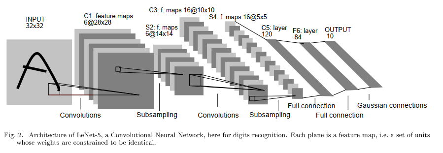
원래 논문에 나왔던 LeNet-5의 구조이다. 이를 코드로 아래와 같이 옮겨 주었다.
    def __init__(self):
        super(Lenet5, self).__init__()
        self.conv1 = nn.Conv2d(1, 6, 5)
        self.conv2 = nn.Conv2d(6, 16, 5)
        self.fc1 = nn.Linear(400, 120)
        self.fc2 = nn.Linear(120, 84)
        self.fc3 = nn.Linear(84,10)
        self.activ = nn.Tanh()
        self.avgpool = nn.AvgPool2d(2)

    def forward(self, x):
        x = self.conv1(x)
        x = self.activ(x*2/3)*1.7159
        x = self.avgpool(x)
        x = self.conv2(x)
        x = self.activ(x*2/3)*1.7159
        x = self.avgpool(x)
        x = x.view(x.size(0), -1)
        x = self.fc1(x)
        x = self.activ(x*2/3)*1.7159
        x = self.fc2(x)
        x = self.activ(x*2/3)*1.7159
        x = self.fc3(x)
        x = self.activ(x*2/3)*1.7159

        return x

my_cnn = Lenet5()
loss_func = nn.CrossEntropyLoss()

optimization = torch.optim.SGD(my_cnn.parameters(), lr = LEARNING_RATE, momentum = MOMENTUM)
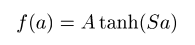
activation function을 github과 달리 위와 같이 정의한 이유는, hyperbolic tangent를 논문과 같이 그대로 이용하기 위함이다. (A = 1.7159, S = 2/3)
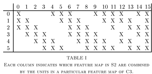
다만, torch에 이미 있는 메소드인 Conv2d를 사용하느라 논문에서 S2에서 C3으로 넘어갈 때 아래와 같이 연결한 건 구현하지 못했고, 전부 연결되어 있는 것으로 생각했다.
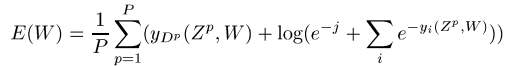
또한, 원래 논문에서는 아래와 같은 MSE loss의 변형을 사용했는데, 구현하기 어려워서 github과 마찬가지로 cross entropy loss를 사용했다.
Training과 오차 계산
training_accuracy = []
validation_accuracy = []

if __name__ == '__main__':
    for epoch in range(NUM_EPOCHS):
        training_loss = 0.0
        num_batches = 0
        for batch_num, training_batch in enumerate(train_loader):
            # split training data into inputs and labels
            inputs, labels = training_batch                              # 'training_batch' is a list
            # wrap data in 'Variable'
            inputs, labels = torch.autograd.Variable(inputs), torch.autograd.Variable(labels)
            # Make gradients zero for parameters 'W', 'b'
            optimization.zero_grad()
            # forward, backward pass with parameter update
            forward_output = my_cnn(inputs)
            loss = loss_func(forward_output, labels)
            loss.backward()
            optimization.step()
            # calculating loss
            training_loss += loss.item()
            num_batches += 1


        print("epoch: ", epoch, ", loss: ", training_loss/num_batches)

        # calculate training set accuracy
        accuracy = 0.0
        num_batches = 0
        for batch_num, training_batch in enumerate(train_loader):        # 'enumerate' is a super helpful function
            num_batches += 1
            inputs, actual_val = training_batch
            # perform classification
            predicted_val = my_cnn(torch.autograd.Variable(inputs))
            # convert 'predicted_val' tensor to numpy array and use 'numpy.argmax()' function
            predicted_val = predicted_val.data.numpy()
            predicted_val = np.argmax(predicted_val, axis = 1)  # retrieved max_values along every row
            # accuracy
            accuracy += accuracy_score(actual_val.numpy(), predicted_val)

        training_accuracy.append(accuracy/num_batches)

        # calculate validation set accuracy
        accuracy = 0.0
        num_batches = 0
        for batch_num, validation_batch in enumerate(valid_loader):        # 'enumerate' is a super helpful function
            num_batches += 1
            inputs, actual_val = validation_batch
            # perform classification
            predicted_val = my_cnn(torch.autograd.Variable(inputs))
            # convert 'predicted_val' tensor to numpy array and use 'numpy.argmax()' function
            predicted_val = predicted_val.data.numpy()
            predicted_val = np.argmax(predicted_val, axis = 1)  # retrieved max_values along every row
            # accuracy
            accuracy += accuracy_score(actual_val.numpy(), predicted_val)
        validation_accuracy.append(accuracy/num_batches)


    epochs = list(range(NUM_EPOCHS))

    # plotting training and validation accuracies
    fig2 = pyplot.figure()
    pyplot.plot(epochs, training_accuracy, 'r')
    pyplot.plot(epochs, validation_accuracy, 'g')
    pyplot.xlabel("Epochs")
    pyplot.ylabel("Accuracy")
    pyplot.show()


    # test the model on test dataset
    correct = 0
    total = 0
    for test_data in test_loader:
        total += 1
        inputs, actual_val = test_data
        # perform classification
        predicted_val = my_cnn(torch.autograd.Variable(inputs))
        # convert 'predicted_val' GPU tensor to CPU tensor and extract the column with max_score
        predicted_val = predicted_val.data
        max_score, idx = torch.max(predicted_val, 1)
        # compare it with actual value and estimate accuracy
        correct += (idx == actual_val).sum()

    print("Classifier Accuracy: ", correct/total * 100)
Training부터는 github에서의 구현을 그대로 썼다. 원래 구현에서는 training, validation, test의 오차를 각각 정의하고, 결과로 test/validation accuracy 그래프와 Classifier accuracy(백 점 만점에서 test의 점수)를 도출했다.
Training 결과
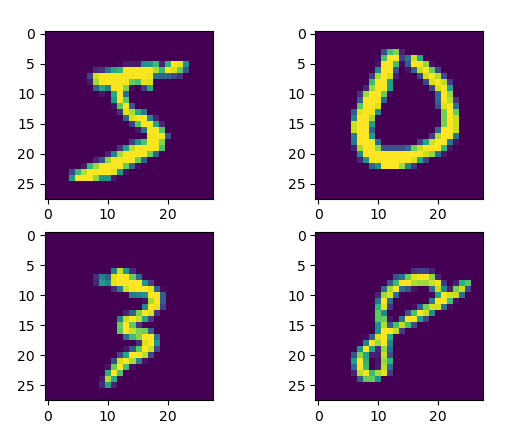
MNIST 손글씨 데이터는 아래와 같이 출력된다.
이 부분은 굳이 필요하지 않아서 내 구현에서는 뺐는데, 필요하다면 github에 들어가서 하면 될 것 같다.
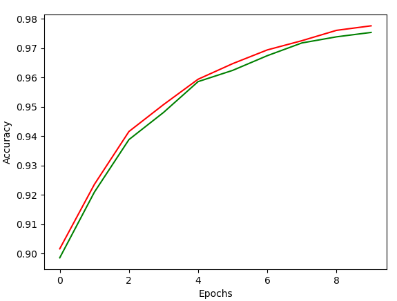
pyplot에 의해 나온 training과 validation 결과이다. 초록색이 validation 결과이며, 빨간색이 training 결과이다. Classifier Accuracy는 97.48점으로 꽤 높은 점수로 나왔다.
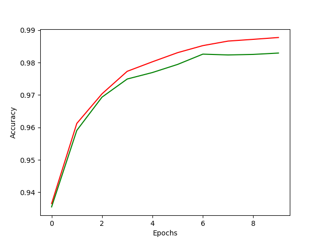
하지만 activation function의 고증을 포기하고, 그냥 tanh 함수를 적용할 경우, 오히려 더 높은 accuracy 값을 보인다.
'머신러닝&딥러닝 > CNN' 카테고리의 다른 글
| U-Net(O. Ronneberger 2015) 논문리뷰 및 pytorch 구현 (0) | 2024.06.25 |
|---|---|
| ImageNet 데이터셋의 AlexNet을 이용한 분류 (A.Krizhevsky 2012 논문 리뷰) (0) | 2024.04.22 |
| CNN에서 backpropagation이 이루어지는 원리 (0) | 2024.03.27 |
| [CNN] LeNet-5를 활용한 손글씨 인식 (Yann LeCun 1998 논문 리뷰) (2) | 2024.02.26 |